Excel Filter

Usage:

Use this formula to filter a range of data (also known as a list or array of data) using single or multiple criteria.

The FILTER formula is perfect for when you want to take a large table of data and extract a small subset of the table using certain rules or specifications.

Function Layout (Syntax):

=FILTER(array, include, [if_empty])

Inputs (Arguments):

• Array: The set of base cells that you want to filter.
• Include: The criteria used to filter the data. This input should be in the form of a boolean equation (which basically means in the form of a yes or no question using “=”, “>”, “<”, etc).
• [If_empty]: This is an optional input. If you fill this in, you can tell Excel to put a value or string of text when the filter returns an empty table. Some common inputs here are empty quotes “ ” or “N/A” or “No Results”.

Example: Single Criteria

Let’s take a look at an example where we filter a range of data based on one criterion or one rule.

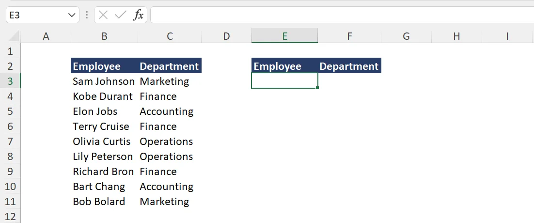
In this particular example, we have a list of employee names and we would like to filter for the employees that work in the finance department. To do this, follow these steps:

1. Initiate the formula by typing “=FILTER(“.
2. Fill in the “array” input. In this case, it should be cells B3:C11.
3. Set up the filter criteria. Here we can type “C3:C11=”Finance”.
4. Then for the third optional step, we can put “N/A” in the case the list changes and we have no finance employees on the list.
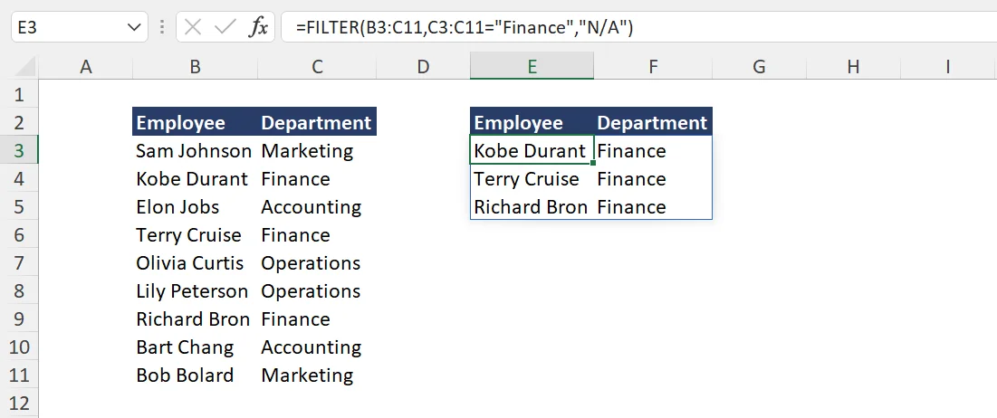
5. Hit enter. You should see a filtered list of finance employees that matches the image below.

=FILTER(B3:C11,C3:C11=”Finance”,”N/A”)

Spill Error

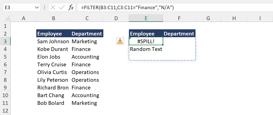
Note: Make sure to leave enough empty cells below for the filtered array. For example, if cell E4 was not empty, you would see a spill error.

Example: Multiple Criteria

So what happens if you need to filter a range with multiple criteria? Well, you can do so pretty easily with some slight adjustments.

Criteria 1 AND Criteria 2

If you want to filter with multiple criteria you’ll need to decide if you need all criteria rules to be true or if you only need one of the criteria rules to be true. If you want all criteria to be true, you can use the * character to divide your rules.

For example, if you want to filter the list below for employees that are in the finance department AND have a salary greater than $80,000, you can use the below formula.

=FILTER(B3:D11,(C3:C11=”Finance”)*(D3:D11>80000),”N/A”)

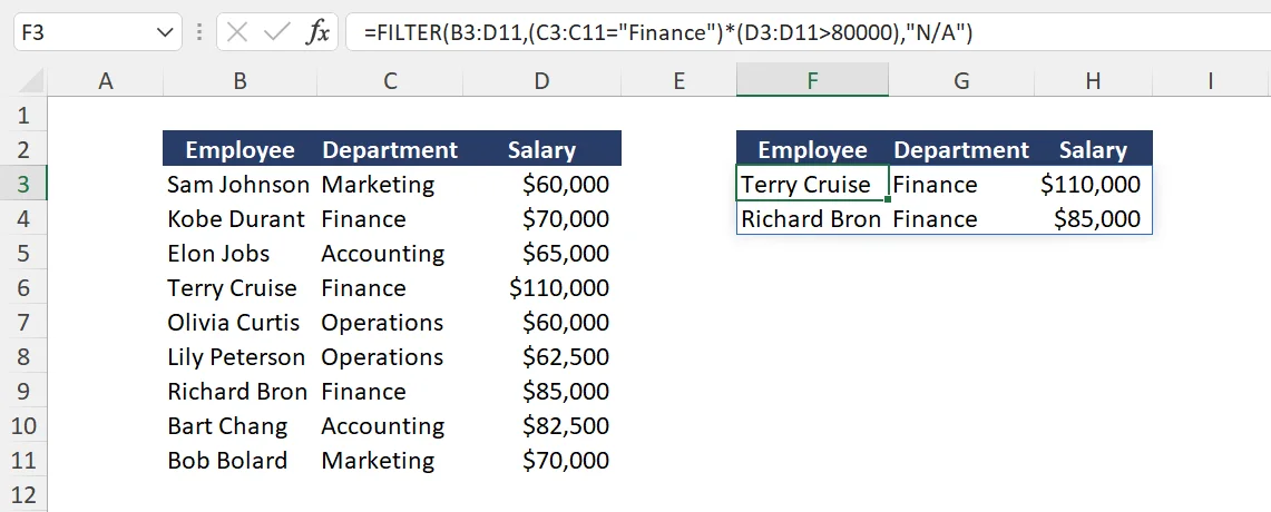
Notice how each criteria rule is contained within a set of parentheses () and they are split by a * symbol. This part of the formula simple translates to: (Rule 1) AND (Rule 2). If you wanted to use more than 2 criteria, simply continue using the same format by stringing on more (criteria) with the * symbol.

Criteria 1 OR Criteria 2

Now instead of AND, what if you only needed criteria 1 OR criteria 2 to be true? Well this can be setup as well.

To do this, simply replace the * symbol with a + symbol. This essentially changes the translated formula from AND to OR.

For example, if we wanted to filter for employees that work in the finance department OR have a salary greater than $80,000, we can use the below formula.

=FILTER(B3:D11,(C3:C11="Finance")+(D3:D11>80000),"N/A")

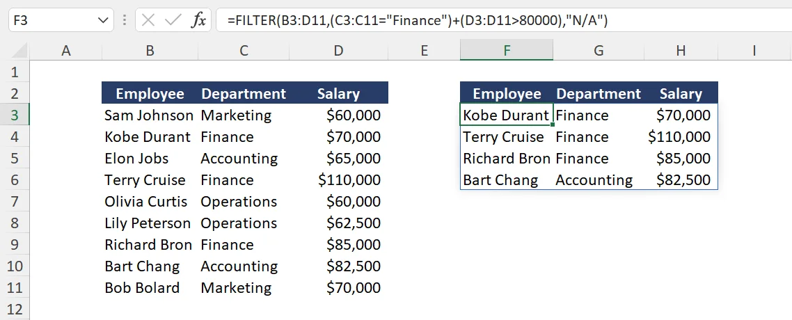
Similar to the previous example, all you need to do is contain your criteria rules in () and separate them with a + symbol. And again, if you need to add more criteria, simply keep the pattern going by adding more (criteria) with + symbols.

Additional Resources

If you’re interested in further developing your Excel skills to better perform in the workplace, check out our Excel for Business & Finance Course and more using the get started button below.

Other Articles You May Find Helpful

• How to Prepare an Income Statement
• Interview with a Tesla Financial Analyst
• Must Know Finance Interview Questions