How to Autofit In Excel

Are you experiencing any of these problems in Excel?

• The cells are displaying “#####” instead of their actual content.
• The cells are not displaying the entire content; it's being cut off.
• Some cells have multiple lines of text, but only one or a few lines are visible.

To fix these issues, you can adjust the column and row sizes. However, doing this manually can be challenging when you have many rows and columns. In such situations, you can easily use the Excel Autofit feature.

How to Autofit Columns in Excel?

You can do autofit columns in Excel in the following ways.

1. Double-click on the column border
2. Use the Format options of the Home tab
3. Use the Excel shortcut Alt + H + O + I

Let’s go through each of the methods. 

Method 1: Double Click on The Column Border

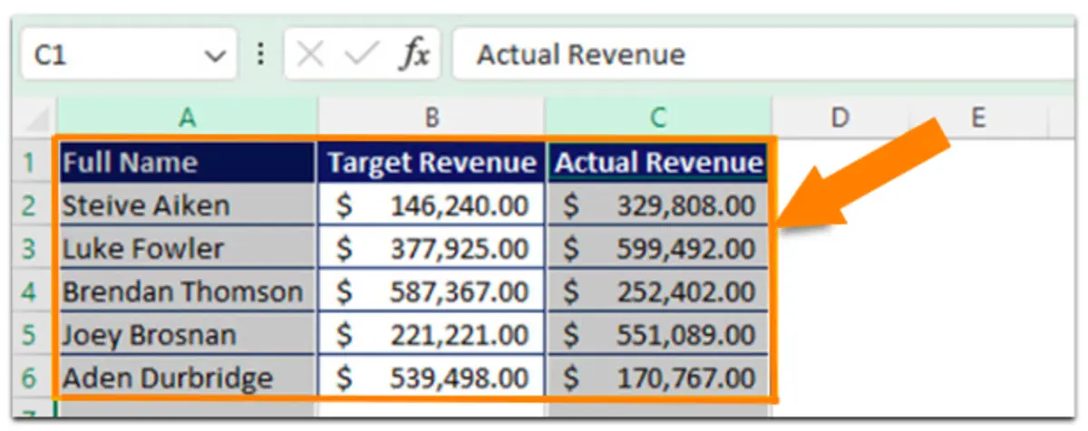
The below table shows the input table for sales achievement calculation.

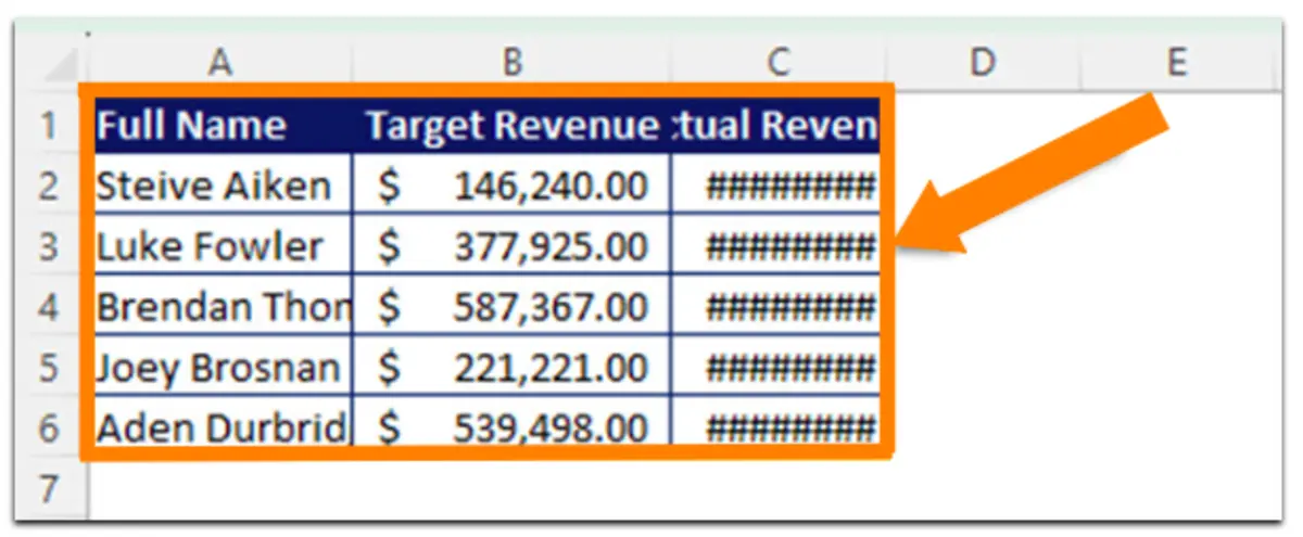
In Column A, some full names are cut off, and in Column C, which holds revenue values, only displays “#####”. To fix these problems, you can use any of the following methods.

To autofit column widths using the double-click method, you have to first select the column or columns in which you want to autofit.
In this scenario, you can choose either Column A and Column C only, or select a range from Column A to Column C. When selecting non-adjacent columns like Column A and Column C, hold down the Ctrl key while clicking on the column headers.

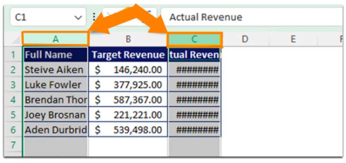
For adjacent columns, begin by selecting the header of the leftmost column, then hold down the Shift key while selecting the header of the rightmost column within the range you want to autofit.

Now move your cursor to the right border of any of the selected columns. You will

notice that the mouse pointer is changing to an icon that has a double-pointed arrow (see image below).

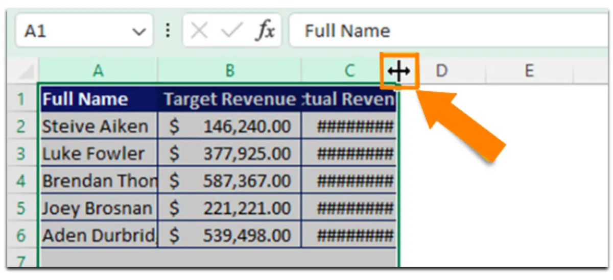
Double-click the trackpad of your laptop or double-click the mouse left button. Now, you have applied the autofit columns to all the selected columns.

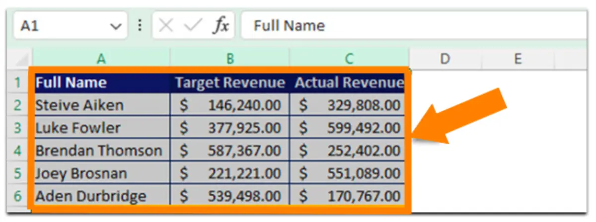
After applying autofit columns, you can see all full names and all the figures in the actual

revenue column. 

Method 2: Format Options

The second method to autofit columns in Excel is to use the format options in the home tab. To do so, follow these steps:

1. First select the column or columns in which you want to autofit.
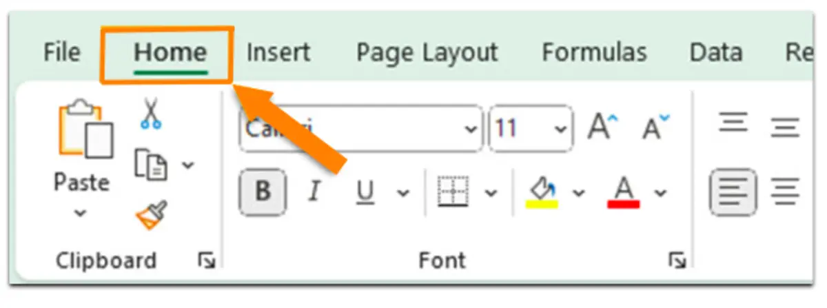
2. Then go to the home tab of your excel ribbon.

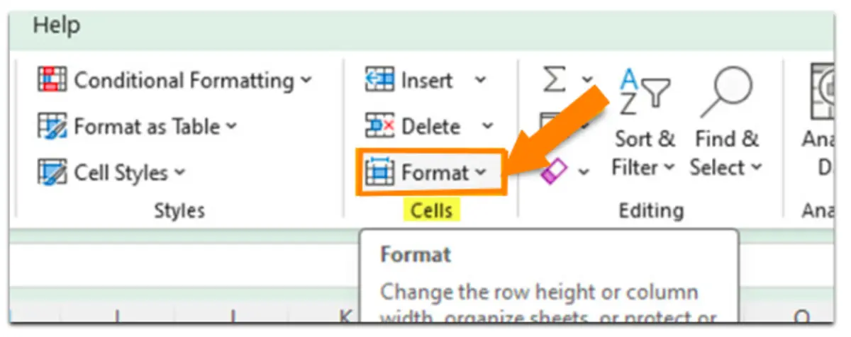
3. Expand the “Format” options in the “Cells” group.

4. Select the “AutoFit Column Width” option from the drop-down list.

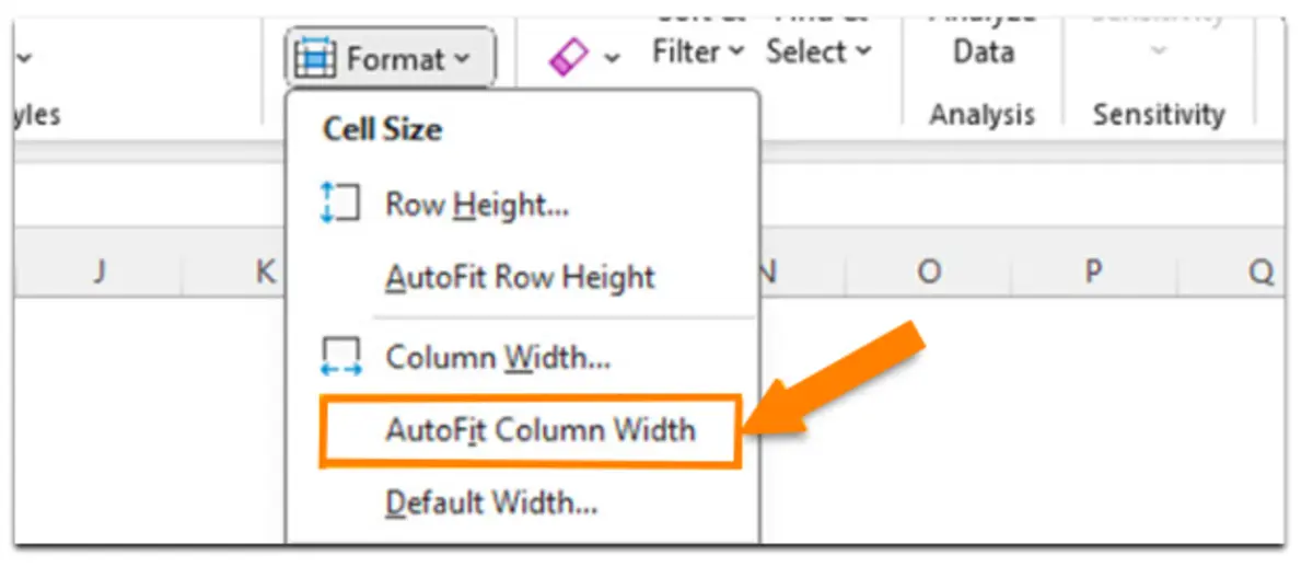
As soon as you select the “AutoFit Column Width” option, Excel autofits all the selected

columns.

Method 3: Use the Excel Shortcut to Autofit Columns

Some Excel users prefer to use Excel shortcuts for their Excel work. If you want to use an

Excel shortcut to autofit columns in Excel, you have to follow the below simple steps.

1. Select the column or columns in which you want to autofit. If you want to select all the columns in your sheet, press Ctrl + A
2. Press the following keys one after the other: Alt + H + O + I
   Don’t try to press all the above keys together. Instead, first press the Alt key. Then, the letter H key, next, the letter O key (not zero), and finally the letter I key.

Now, you will see that the selected columns are getting wider to accommodate the longest.

content in each column.

How to Autofit Rows in Excel?

You can autofit rows in Excel in the following ways:

1. Double-click on the row border
2. Use the Format options of the Home tab
3. Use Excel the shortcut Alt + H + O + A

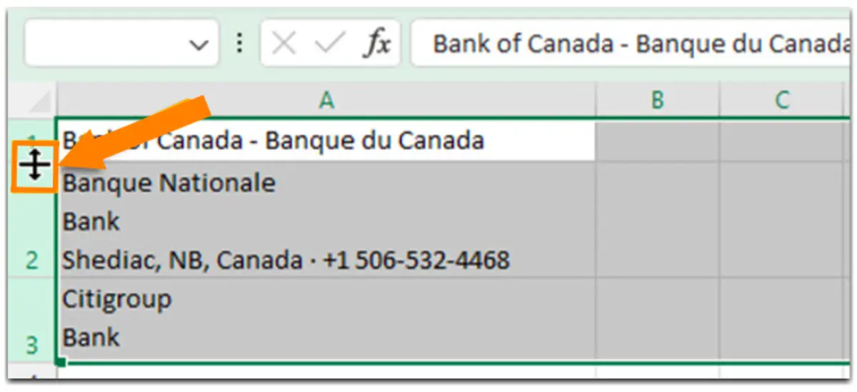
In the image below, Column A displays contact details, with each cell containing multiple lines of text. However, Excel is currently not displaying some of the lines of Row 1 and Row 3.

To fix these problems, you can use any of the following methods.

Method 1: Double Click on The Row Border

To autofit row heights using the double-click method, you have to follow the below steps.

1.  Select the row or rows in which you want to autofit. In this scenario, you can select either Row 1 and Row 3 only or select the entire range of Row 1 to Row 3. When selecting non-adjacent Rows like Row 1 and Row 3, hold down the Ctrl key while clicking on the row headers.
2. Move your cursor to the bottom border of any of the selected rows. You will notice that the mouse pointer is changing to an icon that has a double-pointed arrow.

3. Double-click the trackpad of your laptop or double-click the mouse left button. Now, you have applied the autofit rows to all the selected rows.

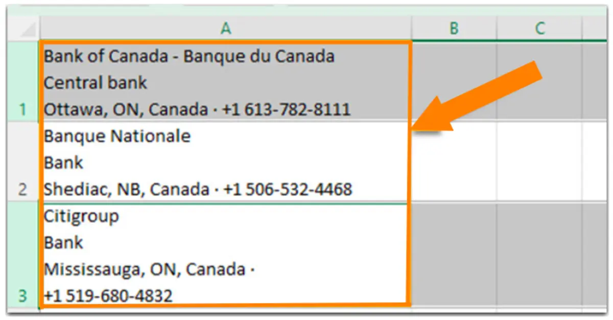
After applying autofit rows, you can see all the full contact details of each cell.

Method 2: Use the Format options of the Home tab to Autofit Rows in Excel

Another method that you can use to apply autofit rows in Excel is by using the Format options of the Home tab. To do that you have to follow the below steps.

1. Select the row or rows that you want to autofit. 
2. Go to the Home tab of your Excel Ribbon.

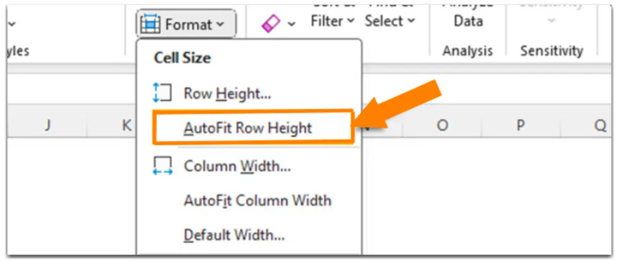
3.  Expand the “Format” options in the “Cells” group.
   

4. Select the “AutoFit Row Height” option from the drop-down list.
   

As soon as you select the “AutoFit Row Height” option, Excel autofits all the selected Rows.

Method 3: Use the Excel Shortcut

Many people who use Excel like to use shortcuts to make their work faster. If you want to

use a shortcut to make rows fit in Excel, you can do it by selecting the relevant rows and pressing the keys: Alt + H + O + A one after the other (not at the same time).

Now, you will see that the selected Rows are getting taller to accommodate the tallest content in each Row.

Practical examples and use cases of Autofit in Excel.

Autofit in Excel is very useful in the following cases.

1. Bulk Data Formatting: This applies when you are dealing with a substantial dataset, and your goal is to ensure that the content in every cell is fully visible.
   
   
2. Formatting Dynamic Data in Excel: This scenario arises when your dataset undergoes frequent updates, and you aim to guarantee that all cell content remains entirely visible.
   
   
3. Imported Data Formatting: This comes into play when you import data from external sources like CSV files, and your objective is to confirm that all cell content is completely visible.

Tips and best practices for optimising Autofit

When employing Excel Autofit feature, keep in mind that it will extend the column width

to fit the longest content in that column. This extension can sometimes disrupt the formatting of your Excel worksheet. Therefore, it's advisable not to use the Autofit option unnecessarily.

Any potential limitations or considerations 

In Excel, columns can hold a maximum of 255 characters in the standard font size, but this

width may decrease if you use larger fonts or apply formatting like italics or bold. The default column width is approximately 8.43 units.

Rows, on the other hand, can have a maximum height of 409 points, where 1 point is

roughly 1/72 inch or 0.035 cm. The default row height varies depending on your screen

settings but is typically around 15 points at 100% dpi and approximately 14.3 points at

200% dpi. These limits are important to consider when formatting your Excel worksheets.

Additional Resources

If you found this article useful, consider checking out our Excel for Business & Finance Course where we help students learn the technical skills needed to perform in competitive finance and investment roles. Use this course to join our students who have landed roles at Goldman Sachs, Amazon, Bloomberg, and other great companies!

Other Articles You Might Find Helpful

• Excel Text To Columns: Learn how to use the Excel Text to Columns tool to split text into one or more cells.
• How to Unhide Columns and Rows in Excel: Learn how to quickly unhide columns and rows in Excel with real examples and suggested alternatives
• Excel ROUNDUP Function: Learn how to use the ROUNDUP function in Excel with usage directions, input directions, input definitions and example use cases.
• Excel Sort Function: Learn how to use the Excel SORT function to sort your data lists, ranges and arrays.