INDEX MATCH with Multiple Criteria
Learn the easy way to perform an INDEX MATCH with multiple criteria in Excel.

Avoid using unnecessarily complex and outdated array formulas to perform an INDEX MATCH using multiple criteria. In this guide, we’ll show you how to use INDEX MATCH on multiple criteria using the ampersand (&) sign in Excel.
INDEX MATCH with Multiple Criteria Excel Formula
=INDEX([array], MATCH([X]&[Y], [array]&[array],0))
To perform an INDEX MATCH with multiple criteria in Excel, simply use an ampersand (&) to place multiple references in your lookup value and lookup array inputs in the MATCH formula.
6 Steps to Performing an INDEX MATCH with Multiple Criteria:
- Initiate the INDEX function and select the base lookup array.
- If searching with row criteria, initiate the MATCH function and input a lookup value, lookup array, and match type.
- If using multiple row criteria, use an ampersand (&) to input secondary lookup values and lookup arrays.
- If searching with column criteria, initiate the MATCH function and input a lookup value, lookup array, and match type.
- If using multiple column criteria, use an ampersand (&) to input secondary lookup values and lookup arrays.
- Close the formula and enter.
The following examples will cover several different multiple criteria lookup scenarios that you might find helpful:
- Multiple Row Criteria INDEX MATCH Lookup
- Multiple Column Criteria INDEX MATCH Lookup
- Advanced Multiple Row & Column INDEX MATCH Lookup
Example 1: Multiple Row Criteria INDEX MATCH Lookup

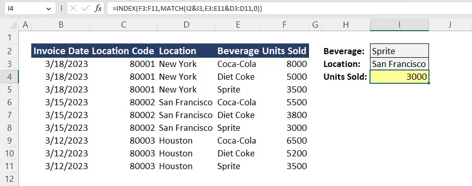
This example spreadsheet contains a basic beverage sales table that shows the units sold by beverage type, location, and invoice date. In this particular example, we’ll show you how to search for a specific row value (units sold) based on 2 different row criteria (beverage name and location).
Step-by-step instructions:
- Initiate the INDEX function and select the base lookup array, which in this case is the column containing the units sold (F3:F11).
- Initiate the MATCH function in the row number input.
- Input both the beverage lookup value (I2) and the location lookup value (I3) within the same lookup input slot and use the ampersand (&) sign to separate the values.
- Input both the beverage lookup array (E3:E11) and the location lookup array (D3:D11) in the same lookup array input slot and use the ampersand (&) sign to separate the arrays. Make sure the arrays are input in the same order as the lookup value inputs.
- Enter zero for an exact match.
- Skip the column number input in the INDEX formula (since we have no column criteria in this example) and close the formula.

Example 2: Multiple Column Criteria INDEX MATCH Lookup

This example spreadsheet breakdowns a company’s sales by historic month and year. In this particular example, we’ll show you how to search for a specific column value (sales) based on 2 different column criteria (year and month).
Step-by-step instructions:
- Initiate the INDEX function and select the base lookup array, which in this case is the row containing the values (B4:J4).
- Skip the row number input since there are no row criteria in this example.
- Initiate the MATCH function in the column number input.
- Input both the year lookup value (M3) and the month lookup value (M4) within the same lookup input slot and use the ampersand (&) sign to separate the values.
- Input both the year lookup array (B2:J2) and the location lookup array (B3:J3) in the same lookup array input slot and use the ampersand (&) sign to separate the arrays. Make sure the arrays are input in the same order as the lookup value inputs.
- Enter zero for an exact match.
- Close the INDEX formula and hit enter.

Example 3: Advanced Multiple Row & Column INDEX MATCH Lookup

This example spreadsheet breakdowns product sales by snack type, team, and month. In this particular example, we’ll show you how to search for a specific table value (sales) based on multiple criteria in both the rows and columns.
Step-by-step instructions:
- Initiate the INDEX function and select the base lookup array, which in this case is the table containing the sales values (C4:K8).
- Initiate the MATCH function in the row number input.
- Input the snack lookup value (N3), the snack lookup array (B4:B8), and zero for an exact match. This is a simple one-criteria MATCH setup.
- Initiate the MATCH function in the column number input.
- Input both the team lookup value (N3) and the month lookup value (N4) within the same lookup input slot and use the ampersand (&) sign to separate the values.
- Input both the team lookup array (C2:K2) and the month lookup array (C3:K3) in the same lookup array input slot and use the ampersand (&) sign to separate the arrays. Make sure the arrays are input in the same order as the lookup value inputs.
- Enter zero for an exact match.
- Close the INDEX formula and hit enter.

Additional Resources
Looking to learn more about Excel? Consider checking out our Excel for Business & Finance Course to learn all the fundamental Excel skills practiced at Fortune 500 companies around the world! Use this course to join our students who have landed roles at Goldman Sachs, Tesla, Amazon, and other top-tier companies.
Other Articles You Might Find Helpful
Ready to Level Up Your Career?
Learn the practical skills used at Fortune 500 companies across the globe.


