How to Freeze Rows and Columns in Excel

Excel users sometimes find themselves scrolling through large data sets in Excel while searching for key figures and calculations. Once you scroll past the default view, you’ll find it useful to be able to freeze certain rows and columns on your screen to make labels and headers easy to reference.

The following will sections will cover the different row and column freezing options in Excel:

• Freeze a row
• Freeze multiple rows
• Freeze a column
• Freeze multiple columns
• Freeze both rows and columns
• Restoring to default view

How to Freeze a Row in Excel

To freeze the top row in Excel, simply go to the view ribbon, select the Freeze Panes dropdown, and select the option for Freeze Top Row. Once activated, you’ll be able to see row 1 at the top of your screen no matter how far down you scroll in the spreadsheet.

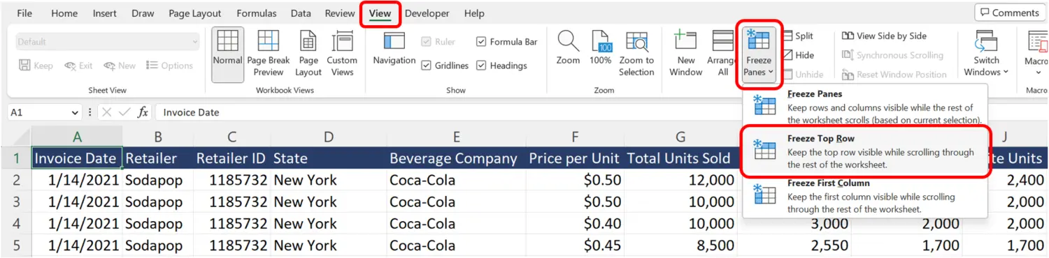
Excel by default, will insert a very subtle thin line below your first row to indicate the end of your frozen section.

How to Freeze Multiple Rows in Excel

Sometimes you’ll want to freeze multiple rows in Excel when you have important label information in more than just the top row in the spreadsheet.

To freeze multiple rows in Excel, select a cell in column A in the row just under your last desired frozen row. Then go to the view ribbon, select the Freeze Panes drop down, and select the Freeze Panes option.

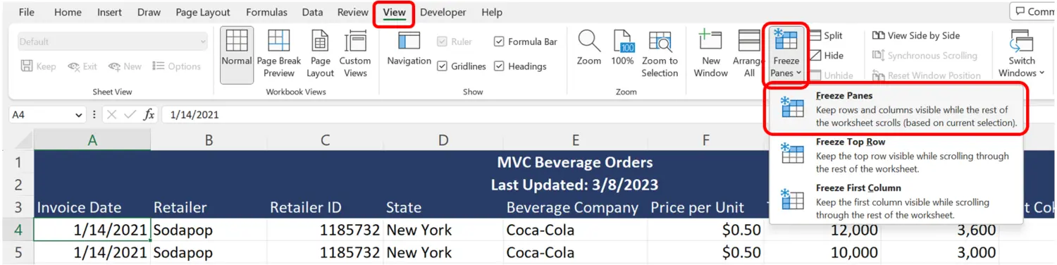
In this particular example, we want to freeze rows 1 to 3. To freeze these rows, select cell A4, then go to view, click the Freeze Panes dropdown, and select Freeze Panes. From here, you’ll be able to see all three of the top rows on your screen as you scroll down the spreadsheet.

Again, you should see a subtle thin line just after row 3 which indicates the row cutoff for frozen panes.

How to Freeze a Column in Excel

To freeze the first column in Excel, click the view ribbon, select the Freeze Panes dropdown, and select the Freeze First Column option. This will freeze column A on your screen so that you can always see the first column (column A) no matter how far right you scroll on your spreadsheet.

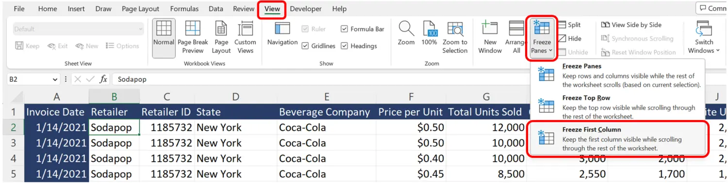
After activation, Excel will put a thin line just after column A to indicate the frozen pane cutoff point just after the first column.

How to Freeze Multiple Columns in Excel

There are some occasions where you’ll want to freeze multiple columns with important reference labels as your scroll horizontally on your spreadsheet.

To freeze multiple columns in Excel, select a cell in row 1 in the column just to the right of the last column that you want to freeze. Then go click on the view ribbon, select Freeze Panes, and select the first option Freeze Panes.

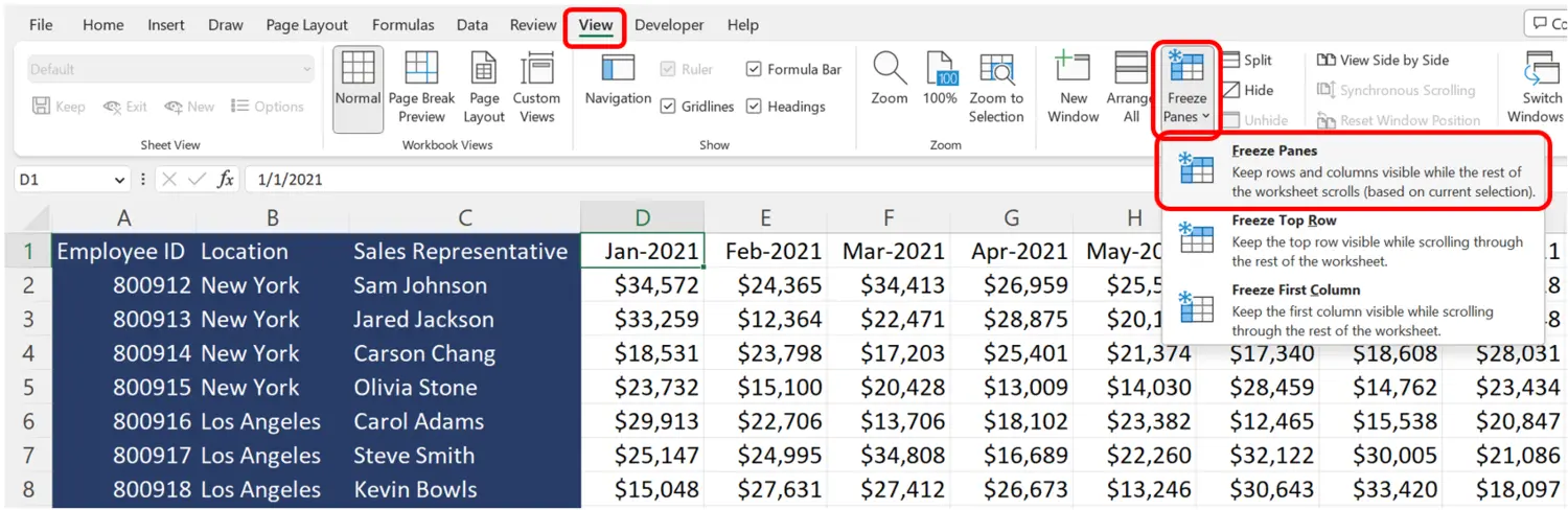
In this particular example, we want to freeze the first 3 columns (Columns A, B, and C). To freeze these columns, select cell D1, then go to view, click the Freeze Panes dropdown, and select Freeze Panes. From here, you’ll be able to see these 3 columns on your screen as you scroll across your spreadsheet.

Again, you should see a subtle thin line just after column C which indicates the column cutoff for frozen panes.

How to Freeze Both Rows and Columns

There will also be cases where you’ll have important labels or descriptive information in both the row headers and the initial columns. In this case, you’ll want to freeze both rows and headers.

To freeze both rows and columns in your Excel sheet, select the cell that is touching your last desired frozen row and last desired frozen column. Then go to view, select the Freeze Panes drop-down, and select the Freeze Panes option.

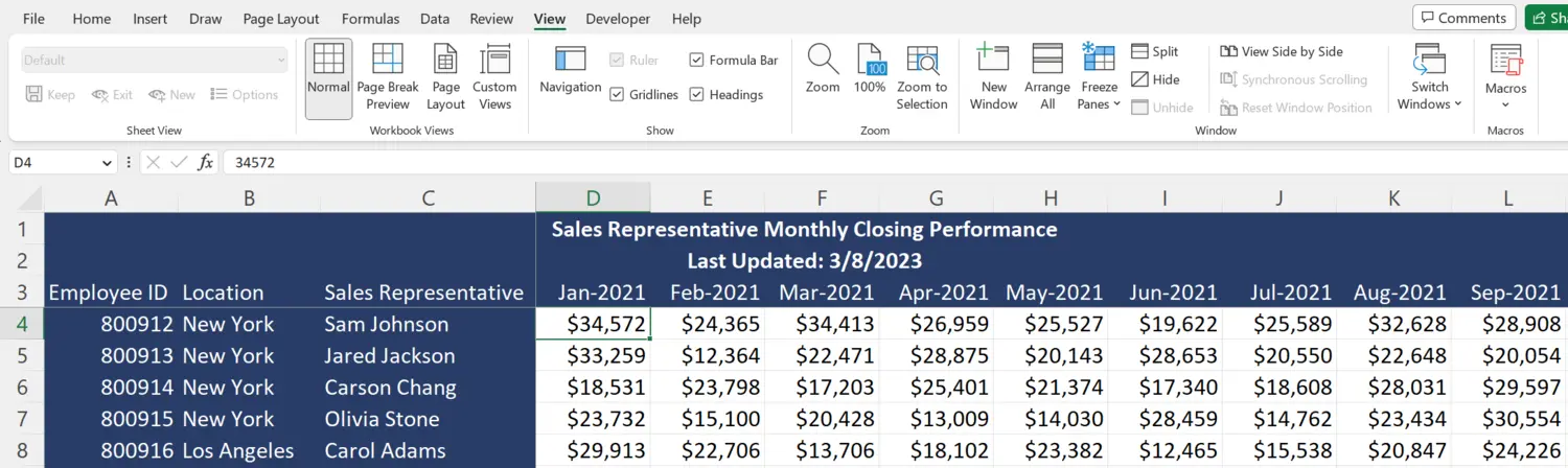
In this particular example, we want to freeze both rows 1 to 3 and columns A to C. To correctly freeze both at the same time, select cell D4 (touching the last desired frozen row and last desired frozen column). From there, go to view, select the Freeze Panes drop-down, and select Freeze Panes. Now you’ll be able to scroll anywhere on your spreadsheet without losing view of these frozen rows and columns.

Restoring to Default View (Removing Frozen Rows and Columns)

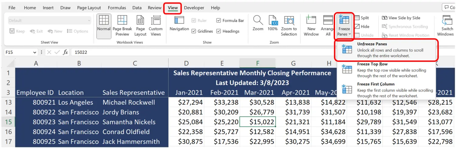
To unfreeze any arrangement of frozen rows or columns, simply go to the view ribbon, open up the Freeze Panes drop-down, and select Unfreeze Panes. This will allow you to freely scroll through the spreadsheet without any fixed rows or columns.

Additional Resources

If you found this article helpful, consider checking out our Excel for Business & Finance Course which features real-world lessons and case studies led by industry professionals. Use this course to join our students who have landed roles at Goldman Sachs, Tesla, Amazon, and other top-tier companies!

Other Articles You May Find Helpful

• The Top 8 Most Important Excel Skills for Finance
• What Does the & Sign Do in Excel
• Excel Data Validation
• Excel Sort Function
• Excel Text to Columns