XLOOKUP Function: Definition and Examples

Excel XLOOKUP Function

The XLOOKUP function looks for a value in a range, and returns the matching result. It works both vertically and horizontally, and can perform several optional arguments such as matching the first or last match, matching an exact match, or the next largest or smallest match.

The Xlookup was introduced in 2019, as a successor to both the VLOOKUP and HLOOKUP functions as it’s able to perform the same actions more efficiently.

Syntax: =XLOOKUP(lookup_value, lookup_array, return_array, [if_not_found],[match_mode],[search_mode]

Breakdown of the inputs (arguments):

• Lookup_value: the value you’re searching for.
• Lookup_array: the range you want to use to find the matching value.
• Return_array: the range containing the corresponding result you want to return.
• [if_not_found]: Optional feature to customize the text if a match is not found.
• [match_mode]: Optional feature to specify the match type (exact match, next smaller item, next larger item, etc.)
• [search_mode]: Optional feature to specify the search mode (starting with the first item on a list, last item on a list, etc.)

Basic Xlookup Example

In the table below, suppose you want to find out the revenue for Brad. Brad can be found in cell C4 and his corresponding revenue is $6,197.

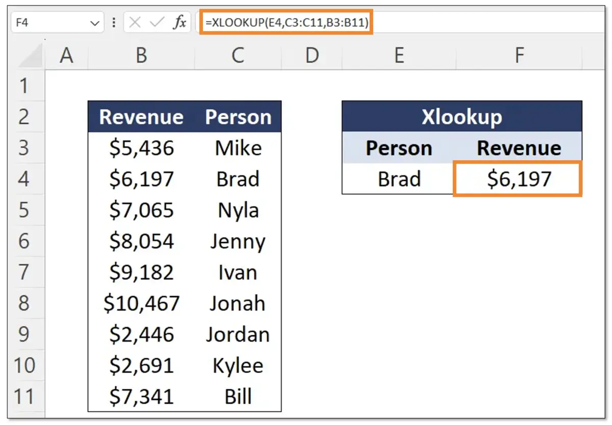
For the Xlookup formula syntax, Lookup_value is cell E4 which is currently Brad. The Lookup_array are cells C3 to C11, which is the person column. The Return_array are cells B3 to B11, which is the revenue column. In this scenario, we don’t need to use any of the Xlookup optional features such as the if_not_found or the match_mode.

You may wonder if the VLOOKUP formula can also find the result. The answer is no because the Vlookup is unable to look for values to the left of the lookup value column. In this case, because the revenue column (column B) is to the left of the person column (column C), it would result in an #N/A sign. For more on Vlookup vs Xlookup, see this article.

Xlookup with If Not Found Example

Using the same table as the example above, suppose we want the result in cell F4 to be “not found” if a person doesn’t appear on the list. For example, suppose we want to find Sara. However, Sara is not found in column C. In this case, we can use the Xlookup if not found feature to specify that Sara is not found on the list.

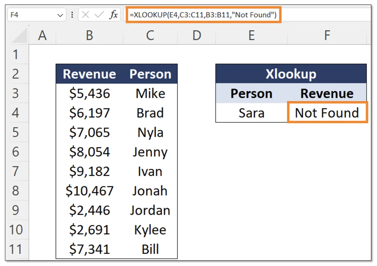
For the Xlookup syntax with the if_not_found feature, after adding the Lookup_value, the Lookup_array, and the Return_array, we want to add the if_not_found by typing our text in quotations. In this case, it’s “Not Found”. When writing text inside a formula, we must always use quotation marks.

Xlookup with Match Mode Example

Using the image below, suppose we want to assign larger discounts the more customers purchase. So a $25 purchase only gets a 3% discount, while a $10,000 purchase gets a 25% discount.

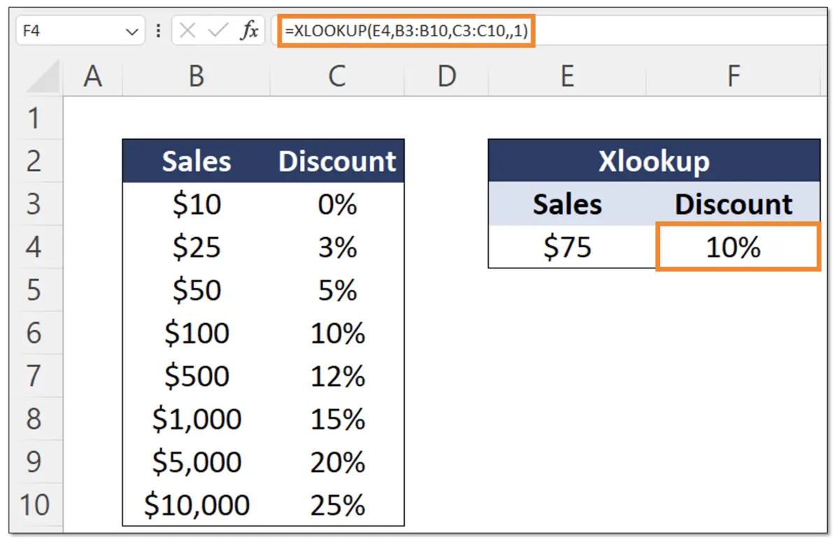
In this scenario, we would like to apply a discount to a $75 purchase. Because $75 is not an option in column B, using the standard Xlookup, we’re going to get an error. To work around this, we need to use the match mode feature on the Xlookup to give us an approximate match. The two options we can use here are:

• Exact match or next smaller item
• Exact match or next larger item

Suppose we go for the latter. The Xlookup syntax is: Lookup_value is E4, lookup_array is B3:B10 (sales column), return_array is C3:C10 (discount column), and because we want to skip the if_not_found feature, we add two commas. Finally, for the match_mode, we chose number 1, which represents the exact match or next larger item.

With this solution, we offer customers a 10% discount for any number greater than $50.

If you’re looking to learn more about Excel formulas, charts & visuals, data analysis, financial modeling, and more, check out our Excel for Business & Finance Course!

Xlookup with Search Mode Example

Referencing the image below, suppose we want to find out the latest revenue for Mike. However, the dataset is in reverse chronological order (oldest to newest). As such, we’re looking for the very last row (row 11), where Mike’s revenue is the most recent.

To work around this, we can use the Xlookup search mode feature. The following options are the most common:

• Search first-to-last
• Search last-to-first

In our case, we want the last-to-first search. The syntax will be: Lookup_value is F4, Lookup_array is B3:B11, Result_array is D3:D11, and we skip both the If_not_found and the Match_mode using commas. Finally, for the Search_Mode, we type -1 which is search last-to-first.

Advanced Xlookup with Multiple Criteria Example

Using the image below, suppose we want to find Mike’s revenue in 2022. Now we have multiple criteria (finding Mike, and finding the year of 2022). For this, we’re going to use an advanced Xlookup feature which is the ampersand (&).

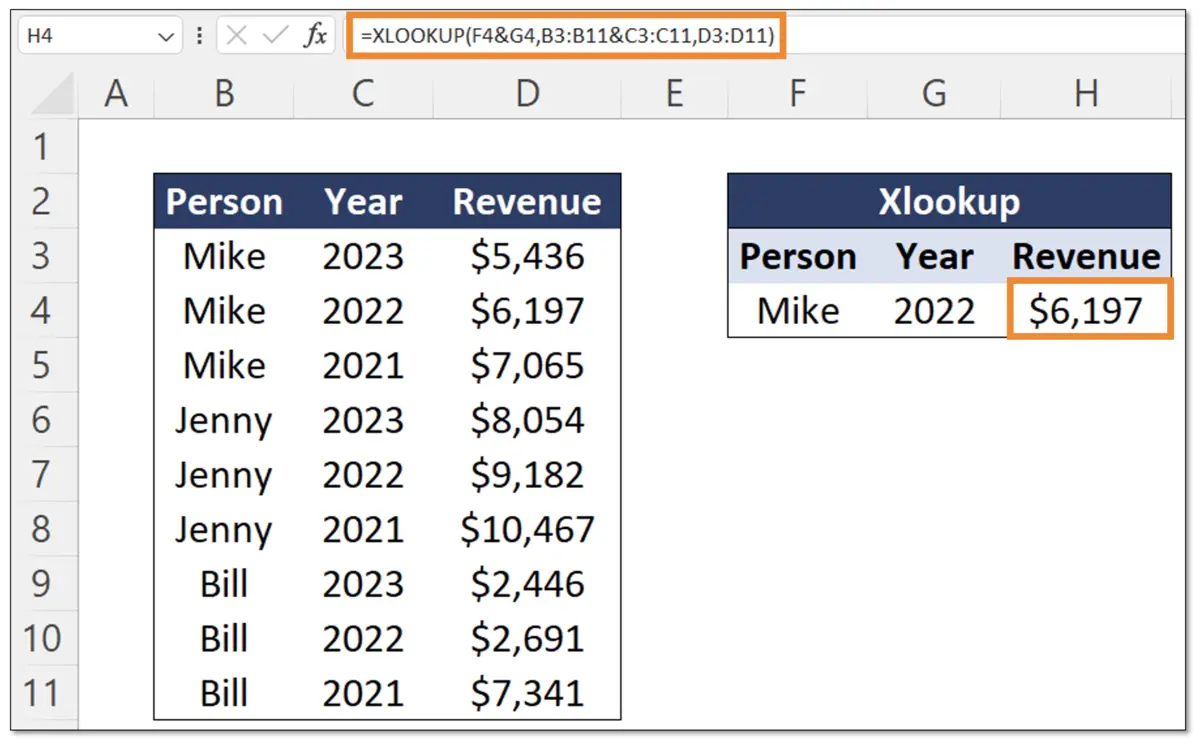
The Xlookup function doesn’t allow for multiple criteria. That’s why we use the ampersand (&) to bypass that limitation. The syntax here is:

• Lookup_value: F4&G4. Because we have two lookup values, we merge them using the ampersand.
• Lookup_array: B3:B11&C3:C11. Just like we have two lookup values, we also have two lookup arrays that we need to merge.
• Return_array: D3:D11. Nothing innovative here, just the result column we’re looking for.  

With this syntax, we’re able to use the Xlookup with multiple criteria to find the revenue for Mike in 2022.

Xlookup vs Index Match

Although the Xlookup is one of the most powerful functions on Excel, it does have some limitations. For example, if we need to look up a value from a table with both column and row headers.

In the scenario below, we’re looking for Mike’s revenue in 2022. The data table is split into a row header with each person’s name (B6:B12) and a column header with the years (C6:E6). Because of the table structure with row and column headers, it is not possible to use a single Xlookup.

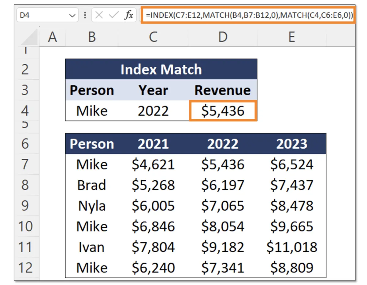
Instead, the better function here is an Index Match. For this, we’ll have an index to capture the whole array, and two match functions to capture both the columns and the rows. The syntax is the following:

• Index(array): this is the range where the output (in our case revenue) lies. So it’s C7:E12
• Row_num: this is our first match, which is for the rows. In our case, this is Mike (B4) as the lookup_value, and all the people (B7:B12) as the lookup_array
• Col_num: this is our second match, which is for columns. In our case, this is 2022 (C4) as the lookup_value, and all of the years (C6:E6) as the lookup_array
• Match_type: For both match functions, we want an exact match

To summarize, the index match combination is better than the Xlookup when you have a table with both row and column headers.

An important note is that the Xlookup is not available in all Excel versions as it is a relatively new function.

Additional Resources

If you want to learn more about Excel, check out our Excel for Business & Finance Course which has helped our students at Goldman Sachs, Bloomberg, Tesla, Amazon, and other top-tier companies.

Other Articles You May Find Helpful

• Xlookup vs Vlookup
• Index Match with Multiple Criteria
• Excel Roundup Function
• Excel Text to Columns
• Excel Sort Function