IFERROR Function in Excel

IFERROR Function Syntax

The IFERROR function returns a value you specify whenever the original output returns an error.

The IFERROR function syntax only has two elements:

• Value: The formula that is checked if it has an error.
• Value_if_error: The custom value you specify if the original formula has an error.

For example, if you want to divide 5/0 and get the answer or a message saying “Bad” if there is an error, then the value is just 5/0, while the value_if_error is “Bad”. In Excel, the syntax for this would be:

=IFERROR(5/0,”Bad”) 

The result here would be the word Bad. This is because 5/0 would give us a #DIV/0! error because we’re trying to divide a number by zero. This would trigger the second argument of value_if_error as the output, hence the Bad as the final output for the formula. 

You may have noticed we use quotations (“”) for the word “Bad”. This is because all text values in an Excel function must always use quotation marks.

Why use the IFERROR function?

The IFERROR function is used to replace an error value on Excel such as an #N/A or a #DIV/0!. Some common examples include:

• #N/A error can occur when you’re looking for a value in a range using a vlookup, xlookup, or index match but that value is not in that range. As Excel can’t find the value in that range, it returns an error sign.
• #DIV/0! error happens when you’re dividing a number by zero. For example, dividing one by zero will return the #DIV/0!. As a workaround, users often add a value_if_error with text saying “N/A” or a numerical value such as a zero.
• Other Excel errors include #VALUE!, #REF!, #NUM!, #NAME?, #NULL!

IFERROR, then blank

If you want the value_if_error to be an empty cell, under the value_if_error write quotation marks with nothing inside like this: “”. This tells Excel you want the value_if_error to be zero. 

As you can see in the example above, the answer with IFERROR is simply an empty cell as we specified the value_if_error to be nothing by adding just quotation marks with nothing in between them.

IFERROR SUM Combination

Although the IFERROR can sometimes be used on its own, it is often combined with another function. This is known as “nesting” a function inside of the first IFERROR argument. For example, below we combine the IFERROR function with the SUM function.

As you can see in the example, we’re trying to SUM cells B2 to B5. However, because we have a #DIV/0! in cell B4, we get an error. To work around this, we used the IFERROR function and added under the value_if_error argument the message “Sum not working” which is currently displaying as the output in cell D3.  

IFERROR VLOOKUP Combination

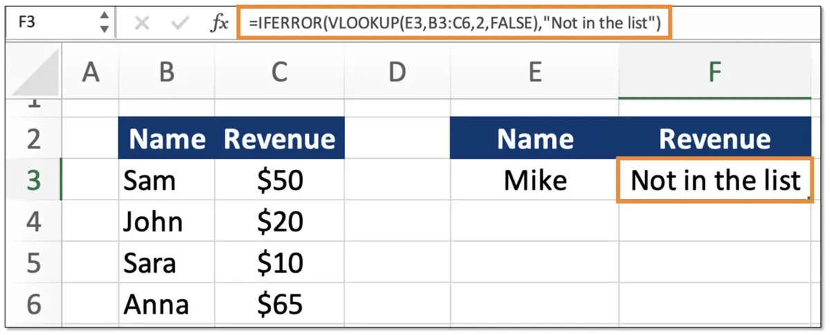
When looking for a value in a range, it is common to use the VLOOKUP function. However, if the VLOOKUP function doesn’t find a value in the specified range, it will return a #N/A error. To work around this, we can combine the IFERROR with the VLOOKUP.

In the example above, we’re looking to find Mike’s revenue in the table range in B2 to C6 using a VLOOKUP. However, as Mike is not on that list, the VLOOKUP would give us an #N/A error. To work around this, we add an IFERROR and nest the VLOOKUP inside the value argument on the IFERROR. Then, as the value_if_error argument, we add the text “not in the list” to explain why we cannot find Mike’s revenue. As Mike is not in the listed range, the output in cell F3 is the message “Not in the list”.

IFERROR XLOOKUP Combination

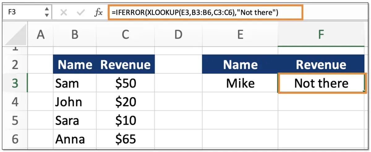
Using an XLOOKUP, we can also consider adding an IFERROR as shown in the image below.

However, the XLOOKUP function has a built-in optional error argument which does the same thing as the IFERROR. This feature is the if_not_found argument in the XLOOKUP. It allows you to customize the text if a match is not found. In other words, it does the same thing as an IFERROR. Therefore, when using the XLOOKUP, it is recommended to use the built-in if_not_found feature as it’s more efficient than combining it with an IFERROR.

IFERROR vs. ISERROR

The ISERROR function is used to just confirm whether a certain value is an error, while the IFERROR function is used to replace an error value with a custom message. 

The ISERROR simply returns a TRUE or FALSE when referring to a specific cell. For example, if the cell value is #N/A it will return a TRUE as it is true that it is an error value. However, if the cell value is 100, it will return a FALSE as it is false that the value 100 is an error.

Additional Resources

If you want to learn more about Excel, check out our Excel for Business & Finance Course which has helped our students at Goldman Sachs, Bloomberg, Tesla, Amazon, and other top-tier companies.

Other Articles You May Find Helpful

• Xlookup Function
• Xlookup vs Vlookup
• Index Match with Multiple Criteria
• Excel Data Validation
• Excel Roundup Function