SUMIFS Function on Excel

SUMIFS Function

The SUMIFS function on Excel sums a range if one or multiple criteria are true. 

=SUMIFS(sum_range, criteria_range1, criteria1,...)

Breakdown of the inputs (arguments):

• Sum_range: the values you want to sum if a condition or multiple conditions are true.
• Criteria_range1: the range that is being tested by criteria1.
• Criteria1: the criteria that defines which values should be added from the criteria_range1.
• … : the three dots at the end of the function represent any additional criteria you might have. To add more criteria, simply put a comma key to activate the next criteria range. The minimum number of criteria is one, while the maximum is 127.

SUMIFS Example With One Criteria

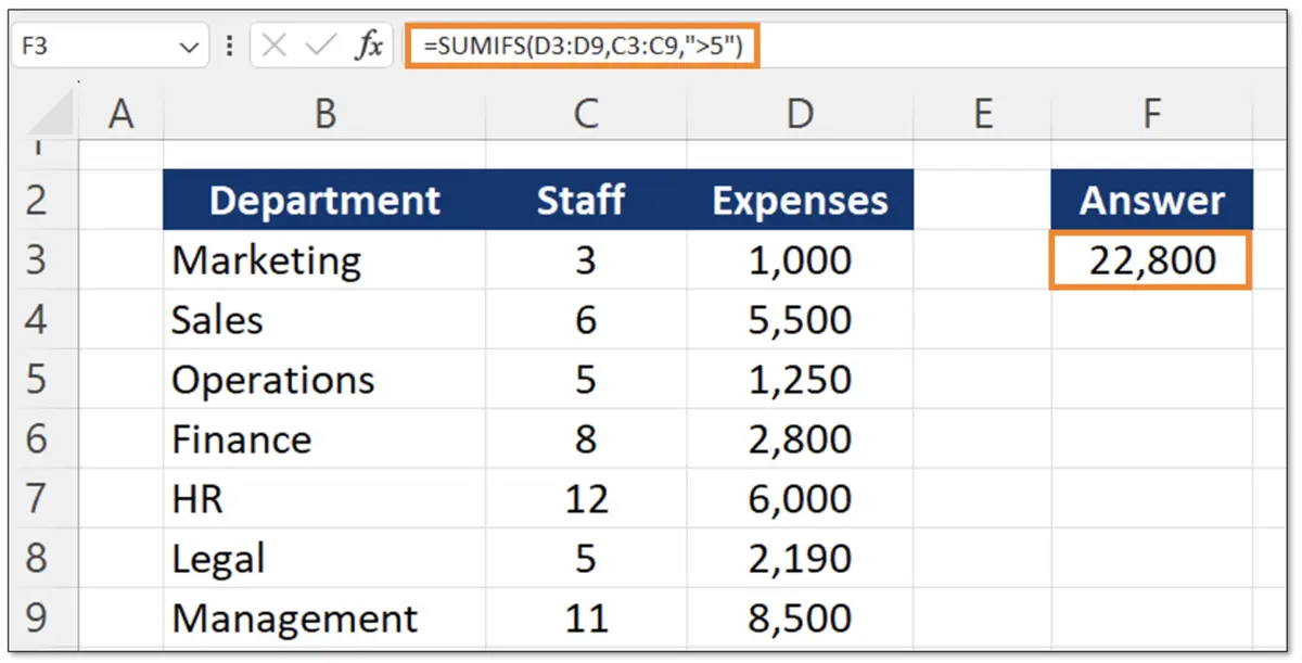
In the table above, we have the expenses by department and the staff count. Suppose we want to find the expenses only for the departments with more than 5 staff. For this, we would use the following formula:

=SUMIFS(D3:D9,C3:C9,”>5”)

• Sum_range: the range with all of the expenses as that’s what we want to sum.
• Criteria_range1: the criteria range we’re interested in (the staff count).
• Criteria1: “>5” (greater than 5) is the criteria that defines how to filter the criteria_range1 so we only sum the expenses with the departments that have more than five people in staff.

For the criteria, it must be wrapped in quotation marks (“”). While we used the greater than operator on this occasion, we can also use equals (=) or the combination of greater than or equal to (>=) as well.  

SUMIFS Example With Two Criteria

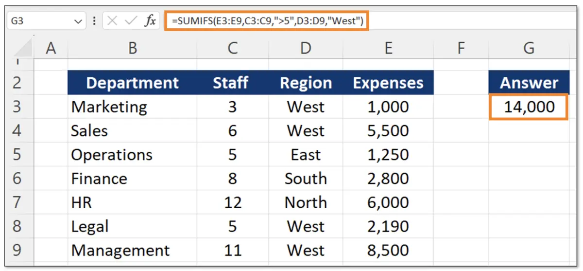
In the image above, we have an example of two criteria. Suppose we want to find the expenses for the departments with more than 5 staff in the West region. We now have two criteria: 

1. > 5 staff
2. West region

For this, we need to use the criteria_range2 and the criteria2. As the criteria_range2 we add the regions in range D3:D9, and also add West in quotation marks as the criteria2.

In this example, we didn’t need an operator like equals or greater than. Instead, we just typed the text we wanted to match (“West”) in quotation marks. 

As for the answer, because of the additional criteria relative to the first example, we now have lower expenses as we’re also filtering by region.

Advanced SUMIFS Example With Wildcard Character 

For an example of an advanced SUMIFS, suppose we want to find out the expenses for Nike where the staff count was greater than 5.

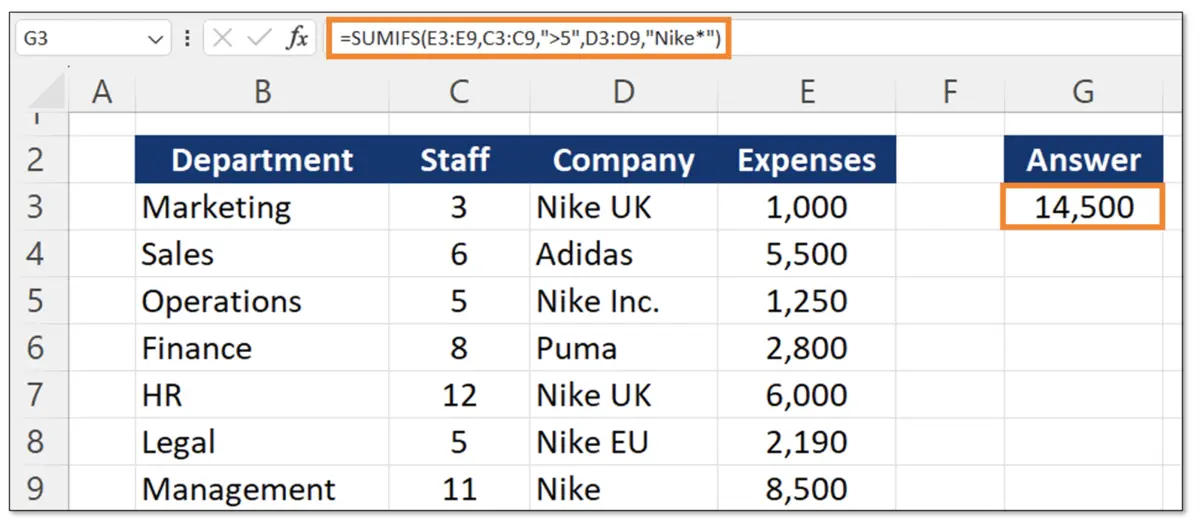
In the image above, under column D for companies, you can see Nike’s name is inconsistent. Sometimes it is Nike UK, other times Nike Inc. and so on. We would like all of these to be considered Nike. 

For this, we can use the wildcard feature by adding an asterisk (*). The asterisk allows for a match to be similar, instead of exact. So as the criteria2, even though we only add Nike followed by an asterisk (“Nike*”) it still matches with Nike EU, Nike UK, etc. In other words, it matches with anything that starts with Nike.   

The SUMIFS with an asterisk also works from the opposite side. So instead of Nike followed by an asterisk (Nike*), we could also do asterisk followed by Nike (*Nike) to pick up any values that end with Nike instead of start with Nike. 

Overall, the asterisk is useful when you forget a person’s first or last name, how their email address ends, or how their phone number starts.

Nested SUMIFS?

While the SUMIFS function may seem extensive, you may sometimes need to merge it with another function. This is known as nesting on Excel. For example, if you want to prevent a #DIV/0! error, it is best practice to use the IFERROR function by nesting the SUMIFS function inside of it. 

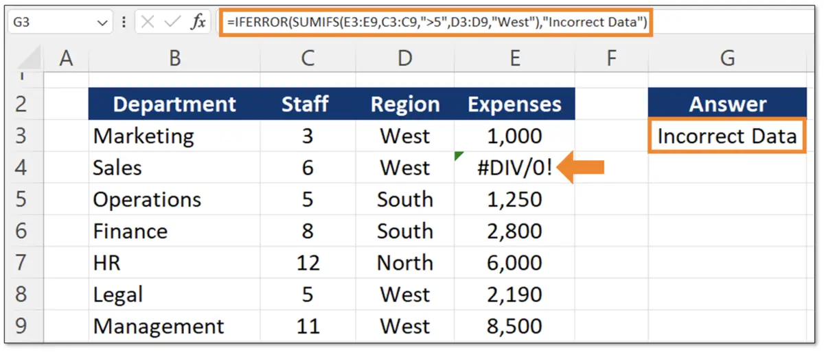
In the image above, we have a #DIV/0! error in cell E4 under the expenses. If we just leave the SUMIFS function, it also returns a  #DIV/0! error because of the error in the original data (cell E4). To work around this problem, we can nest the SUMIFS inside of the IFERROR function. Below are the set of steps:

1. In the formula bar, after the equals sign (=) and before the SUMIFS, add the IFERROR function.
2. At the end of the SUMIFS function, add a comma key to activate the IFERROR function.
3. As the value_if_error, add the text “incorrect data” in quotation marks so users understand there is a problem with the original data and not with the function.

SUMIFS Not Working

The SUMIFS function may not work due to several reasons. Among them are the following:

1. Range sizes are not consistent: The ranges for a SUMIFS must be the same size. For example, if the sum_range is 5 rows and 1 column, then the criteria_range1 and all other criteria ranges must also be 5 rows and 1 column.
2. Errors in the original data: If the original data has errors such as #DIV/0! or #VALUE!, then the SUMIFS function will output an error message as it will not be able to sum the values.
3. Numbers are formatted as text: The SUMIFS function will be incorrect if the values it has to sum are formatted as text instead of as numbers.

SUMIFS vs SUMIF

The SUMIF function only works for one criteria, while the SUMIFS function works for one or multiple criteria. Overall, we recommend always using the SUMIFS instead of the SUMIF as it’s more flexible for editing (like adding more criteria later) and generally has a simpler syntax than the SUMIF.

Additional Resources

For more on Excel, check out our Excel for Business & Finance Course which has helped our students at Goldman Sachs, Bloomberg, Tesla, Amazon, and other top-tier companies.

Other Articles You Might Find Helpful

• IFERROR Function
• XLOOKUP Function
• XLOOKUP vs VLOOKUP
• INDEX MATCH with Multiple Criteria
• ROUNDUP Function