Count Unique Values in Excel

Method 1: UNIQUE and COUNTA Functions

The simplest method to count unique values in Excel uses the UNIQUE and COUNTA functions.

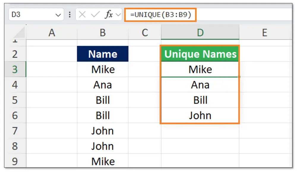
The UNIQUE function returns a list of unique values from a specified range. For example, in the table below, where the names Bill, Mike, and John are duplicated, by using the UNIQUE function we’re able to filter them out of the results table.

Now that we have the unique values, we need to count them, which we can do using the COUNTA function. This function counts the number of non-empty cells in a range. As you can see below, we add the COUNTA function in front of the UNIQUE function. This formula works by first generating a list of unique values using the UNIQUE function and then counting those unique values with the COUNTA function.

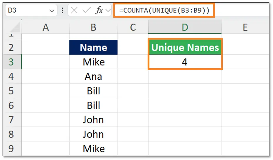
=COUNTA(UNIQUE(A2:A10))

With this method, we managed to count the unique values in Excel. Unfortunately, the UNIQUE function is only available for Excel 2019 and later versions. So if you use an earlier version of Excel, here’s an alternative solution.

Method 2: SUMPRODUCT and COUNTIF Functions

The second method for counting unique values in Excel uses the SUMPRODUCT and COUNTIF functions.

The COUNTIF function counts the number of cells within a range that meet a specific condition. In this case, we’ll use it to count the number of times each value appears in a range.

COUNTIF Function Syntax: COUNTIF(range, criteria)

Where the range is the range of cells to evaluate and the criteria is the condition to count, which in this case is each value in the range itself.

As you can see in the table above, the COUNTIF(B3:B9,B3:B9) counts how many times each value B3:B9 appears within the same range.

To focus on unique values, you calculate the reciprocal (1 divided by the count) of each element in the COUNTIF array. This turns each count into a fraction where duplicates contribute less to the sum. So instead of having 1 or 2, we now have 1 or 0.5.

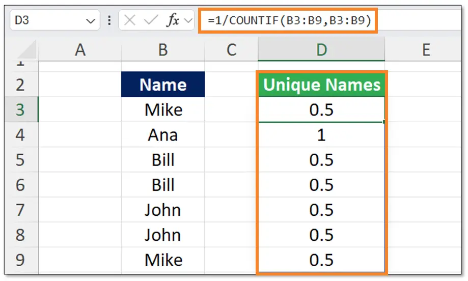
The next step is to use the SUMPRODUCT function to sum up the array of reciprocals. Each unique value will contribute exactly 1 to the sum because its reciprocal is 1. Duplicates will contribute less than 1 because their reciprocals are fractions.

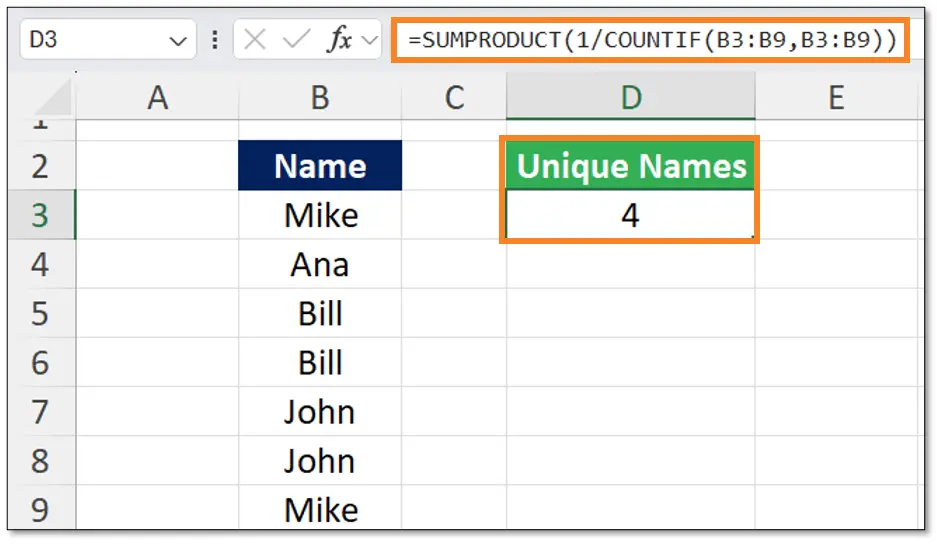
=SUMPRODUCT(1/COUNTIF(B3:B9, B3:B9))

To summarize:

• COUNTIF(B3:B9,B3:B9): Counts occurrences of each value in the range B3:B9.
• 1 / COUNTIF(B3:B9,B3:B9): Computes the reciprocal of each count.
• SUMPRODUCT(…): Sums these reciprocals to get the total count of unique values.

Method 3: Pivot Tables

The third method to count unique values in excel is to use a Pivot Table. For this, select your data range, and go to the insert tab, and click on PivotTable. In the Create PivotTable dialog box, ensure the correct range is selected. Choose where you want the PivotTable to be placed (e.g., New Worksheet or Existing Worksheet). Make sure you tick on “Add this data to the Data Model” in the popup.

Once the pivot table is set up, drag the field that contains the values you want to count (in this case the names) into the Rows area. Then Drag the same field into the values area. See the image below for reference.

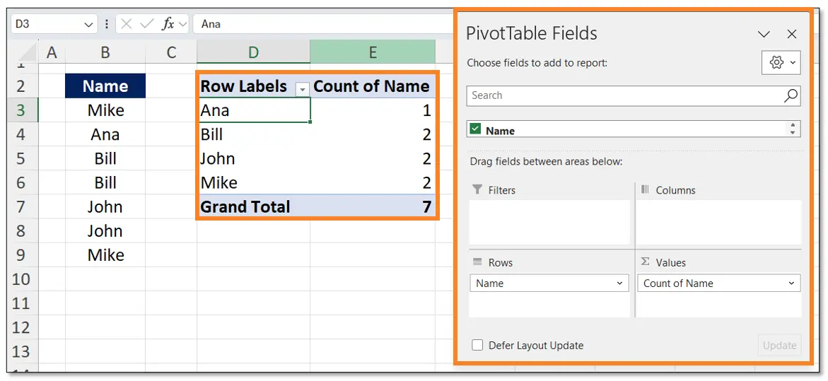
Currently, it’s giving us the total count, instead of the unique count. To count unique values, click on the drop-down arrow next to the field in the Values area (in this case “Count of Name” and select Value Field Settings.

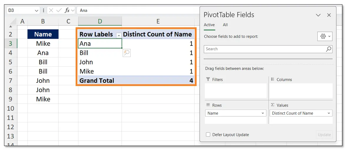
In the Value Field Settings dialog box, choose Distinct Count and this will return the count of unique values. As you can see below, we have the same result for the count of unique values as the first and second method.

Additional Resources

If you found this article useful, consider checking out our Excel for Business & Finance Course where our students have landed roles at Goldman Sachs, Amazon, Bloomberg, and other great companies!

Other Articles You Might Find Helpful

• SUMIFS Function
• XLOOKUP Function
• IFERROR Function
• GROUPBY Function
• COUNTIFS Function